NOTE: THIS DOCUMENT IS OBSOLETE, PLEASE CHECK THE NEW VERSION: "Mathematics of the Discrete Fourier Transform (DFT), with Audio Applications --- Second Edition", by Julius O. Smith III, W3K Publishing, 2007, ISBN 978-0-9745607-4-8. - Copyright © 2017-09-28 by Julius O. Smith III - Center for Computer Research in Music and Acoustics (CCRMA), Stanford University
<< Previous page TOC INDEX Next page >>
Appendix A: Round-Off Error Variance
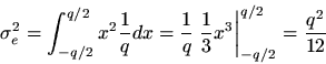
This section shows how to derive that the noise power of quantization error is
, where
is the quantization step size.
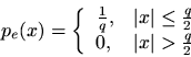
Each round-off error in quantization noise
is modeled as a uniform random variable between
and
. It therefore has the probability density function (pdf)
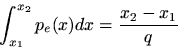
Thus, the probability that a given roundoff erroris given by
assuming of course thatand
lie in the allowed range
. We might loosely refer to
as a probability distribution, but technically it is a probability density function, and to obtain probabilities, we have to integrate over one or more intervals, as above. We use probability distributions for variables which take on discrete values (such as dice), and we use probabilitydensities for variables which take on continuous values (such as round-off errors).
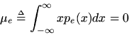
The mean of a random variable is defined as
In our case, the mean is zero because we are assuming the use ofrounding (as opposed to truncation, etc.).The mean of a signal
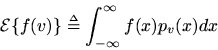
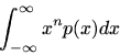
. In general, the expected value of any function
of a random variable
is given by
Since the quantization-noise signal
Probability distributions are often be characterized by theirmoments. The
th moment of the pdf
is defined as
Thus, the meanis the first moment of the pdf. The second moment is simply the expected value of the random variable squared, i.e.,
.
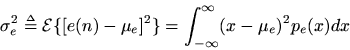
The variance of a random variable
''Central'' just means that the moment is evaluated after subtracting out the mean, that is, looking atinstead of
Note that the variance ofover time, that is, by computing the mean square. Such an estimate is called the sample variance. For sampled physical processes, the sample variance is proportional to the average power in the signal. Finally, the square root of the sample variance (the rms level) is sometimes called the standard deviation of the signal, but this term is only precise when the random variable has a Gaussian pdf.
EE 278 is the starting course on statistical signal processing at Stanford if you are interested in this and related topics. A good text book on the subject is [13].