NOTE: THIS DOCUMENT IS OBSOLETE, PLEASE CHECK THE NEW VERSION: "Mathematics of the Discrete Fourier Transform (DFT), with Audio Applications --- Second Edition", by Julius O. Smith III, W3K Publishing, 2007, ISBN 978-0-9745607-4-8. - Copyright © 2017-09-28 by Julius O. Smith III - Center for Computer Research in Music and Acoustics (CCRMA), Stanford University
<< Previous page TOC INDEX Next page >>
Graphical Convolution
Note that the cyclic convolution operation can be expressed in terms of previously defined operators as
whereand
. It is instructive to interpret the last expression above graphically.
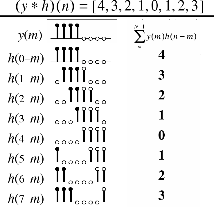
Figure 8.3 illustrates convolution of
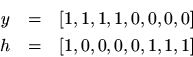
For example,could be a ''rectangularly windowed signal, zero-padded by a factor of 2,'' where the signal happened to be dc (all
s). For the convolution, we need
which is the same as, we say that
ismatched filter for
. The zero-paddingserves to simulate acyclic convolution using circular convolution. The figure illustrates the computation of the convolution of
Note that a large peak is obtained in the convolution output at time. This large peak (the largest possible if all signals are limited to
in magnitude), indicates the matched filter has ''found'' the dc signal starting at time

![$y=[1,1,1,1,0,0,0,0]$](https://technick.net/img/guide_dft/img28.png) and its ''
and its '' ).
).