NOTE: THIS DOCUMENT IS OBSOLETE, PLEASE CHECK THE NEW VERSION: "Mathematics of the Discrete Fourier Transform (DFT), with Audio Applications --- Second Edition", by Julius O. Smith III, W3K Publishing, 2007, ISBN 978-0-9745607-4-8. - Copyright © 2017-09-28 by Julius O. Smith III - Center for Computer Research in Music and Acoustics (CCRMA), Stanford University
<< Previous page TOC INDEX Next page >>
DB for Display
In practical signal processing, it is common to choose the maximum signal magnitude as the reference amplitude. That is, we normalize the signal so that the maximum amplitude is defined as 1, or 0 dB. This convention is also used by ''sound level meters'' in audio recording. When displaying magnitude spectra, the highest spectral peak is often normalized to 0 dB. We can then easily read off lower peaks as so many dB below the highest peak.
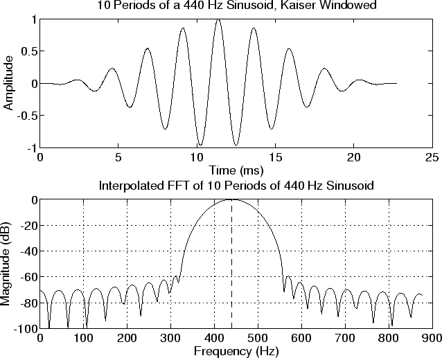
Figure 4.1b shows a plot of the Fast Fourier Transform (FFT) of ten periods of a ''Kaiser-windowed'' sinusoid at
Hz. (FFT windowswill be discussed later in this course. For now, just think of the window as selecting and tapering a finite-duration section of the signal.) Note that the peak dB magnitude has been normalized to zero, and that the plot has been clipped at -100 dB.
Below is the Matlab code for producing Fig. 4.1. Note that it contains several elements (windows, zero padding, spectral interpolation) that we will not cover until later. They are included here as ''forward references'' in order to keep the example realistic and practical, and to give you an idea of ''how far we have to go'' before we know how to do practical spectrum analysis. Otherwise, the example just illustrates plotting spectra on an arbitrary dB scale between convenient limits.
% Example practical display of the FFT of a synthesized sinusoid

fs = 44100;             % Sampling rate
f = 440;                % Sinusoidal frequency = A-440
nper = 10;              % Number of periods to synthesize
dur = nper/f;           % Duration in seconds
T = 1/fs;               % Sampling period
t = 0:T:dur;            % Discrete-time axis in seconds
L = length(t)           % Number of samples to synthesize
ZP = 5;                 % Zero padding factor (for spectral interpolation)
N = 2^(nextpow2(L*ZP))  % FFT size (power of 2)

x = cos(2pift);      % A sinusoid at A-440 (a “row vector”)
w = kaiser(L,8);        % We’ll learn a bit about “FFT windows” later
xw = x . w’;           % Need to transpose w to get a row vector
sound(xw,fs);           % Might as well listen to it
xzp = [xw,zeros(1,N-L)];% Zero-padded FFT input buffer
X = fft(xzp);           % Spectrum of xw, interpolated by factor ZP

Xmag = abs(X);          % Spectral magnitude
Xdb = 20*log10(Xmag);   % Spectral magnitude in dB

XdbMax = max(Xdb);      % Peak dB magnitude
Xdbn = Xdb - XdbMax;    % Normalize to 0dB peak

dBmin = -100;           % Don’t show anything lower than this
Xdbp = max(Xdbn,dBmin); % Normalized, clipped, dB magnitude spectrum
fmaxp = 2f;            % Upper frequency limit of plot, in Hz
kmaxp = fmaxpN/fs;     % Upper frequency limit of plot, in bins
fp = fs*[0:kmaxp]/N;    % Frequency axis in Hz

% Ok, plot it already!

subplot(2,1,1);
plot(1000*t,xw);
xlabel(‘Time (ms)’);
ylabel(‘Amplitude’);
title(sprintf(‘a) %d Periods of a %3.0f Hz Sinusoid, Kaiser Windowed’,nper,f));

subplot(2,1,2);
plot(fp,Xdbp(1:kmaxp+1)); grid;
% Plot a dashed line where the peak should be:
hold on; plot([440 440],[dBmin,0],’–’); hold off;
xlabel(‘Frequency (Hz)’);
ylabel(‘Magnitude (dB)’);
title(sprintf(‘b) Interpolated FFT of %d Periods of %3.0f Hz Sinusoid’,nper,f));
The following more compact Matlab produces essentially the same plot, but without the nice physical units on the horizontal axes:
x = cos([0:2pi/20:102pi]); % 10 periods of a sinusoid, 20 samples/cycle
L = length(x);
xw = x’ . kaiser(L,8);
N = 2^nextpow2(L*5);
X = fft([xw’,zeros(1,N-L)]);

subplot(2,1,1); plot(xw);
xlabel(‘Time (samples)’); ylabel(‘Amplitude’);
title(‘a) 10 Periods of a Kaiser-Windowed Sinusoid’);

subplot(2,1,2); kmaxp = 2105; Xl = 20log10(abs(X(1:kmaxp+1)));
plot([105+1,10*5+1],[-100,0],[0:kmaxp],max(Xl - max(Xl),-100)); grid;
xlabel(‘Frequency (Bins)’); ylabel(‘Magnitude (dB)’);
title(‘b) Interpolated FFT of 10 Periods of Sinusoid’);
