Example 1: FFT of a Simple Sinusoid

NOTE: THIS DOCUMENT IS OBSOLETE, PLEASE CHECK THE NEW VERSION: "Mathematics of the Discrete Fourier Transform (DFT), with Audio Applications --- Second Edition", by Julius O. Smith III, W3K Publishing, 2007, ISBN 978-0-9745607-4-8. - Copyright © 2017-09-28 by Julius O. Smith III - Center for Computer Research in Music and Acoustics (CCRMA), Stanford University

<< Previous page  TOC  INDEX  Next page >>

Example 1: FFT of a Simple Sinusoid

Our first example is an FFT of the simple sinusoid

where we choose (frequency ) and (sampling rate set to 1). Since we're using the FFT, the signal length must be a power of . Here is the Matlab code:

echo on; hold off; diary off;
% !/bin/rm -f examples.dia; diary examples.dia    % For session log
% !mkdirs eps                                     % For figures

% Example 1: FFT of a DFT sinusoid

% Parameters:
N = 64;               % Must be a power of two
T = 1;                % Set sampling rate to 1
f = 0.25;             % Sinusoidal frequency in cycles per sample
A = 1;                % Sinusoidal amplitude
phi = 0;              % Sinusoidal phase
n = [0:N-1];
x = cos(2pinfT);  % Signal to analyze
X = fft(x);           % Spectrum

Let’s plot the time data and magnitude spectrum:

% Plot time data
figure(1);
subplot(3,1,1);
plot(n,x,’’);     

ni = [0:.1:N-1];      % Interpolated time axis
hold on;
plot(ni,cos(2pinif*T),’-’);
title(‘Sinusoid Sampled at 1/4 the Sampling Rate’);
xlabel(‘Time (samples)’); ylabel(‘Amplitude’);
text(-8,1,‘a)’);

% Plot spectral magnitude
magX = abs(X);
fn = [0:1.0/N:1-1.0/N];  % Normalized frequency axis
subplot(3,1,2);
stem(fn,magX)
xlabel(‘Normalized Frequency (cycles per sample))’);
ylabel(‘Magnitude (Linear)’);
text(-.11,40,‘b)’);

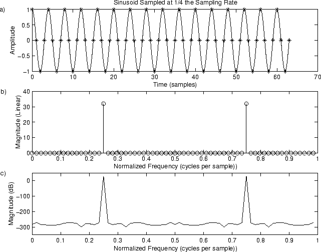
% Same thing on a dB scale
spec = 20*log10(magX);  % Spectral magnitude in dB
subplot(3,1,3);
plot(fn,spec);
axis([0 1 -350 50]);
xlabel(‘Normalized Frequency (cycles per sample))’);
ylabel(‘Magnitude (dB)’);
text(-.11,50,‘c)’);
print -deps eps/example1.eps; hold off;

Figure 9.1:Sampled sinusoid at . a) Time waveform. b) Magnitude spectrum. c) DB magnitude spectrum.

The results are shown in Fig. 9.1. The time-domain signal is shown in Fig. 9.1a, both in pseudo-continuous and sampled form. In Fig. 9.1b, we see two peaks in the magnitude spectrum, each at magnitude on a linear scale, located at normalized frequencies and . Since the DFT length is , a spectral peak amplitude of is what we expect, since

when <img width=“73” height=“28” align=“MIDDLE” border=“0” src="/img/guide_dft/img1379.png" alt="$" mega="" pm\omega="" x="" />. This happens at bin numbers and for . However, recall that Matlab requires indexing from , so that these peaks will really show up at index and in the magX array.

The spectrum should be exactly zero at the other bin numbers. How accurately this happens can be seen by looking on a dB scale, as shown in Fig. 9.1c. We see that the spectral magnitude in the other bins is on the order of dB lower, which is close enough to zero for audio work.

<< Previous page  TOC  INDEX  Next page >>