Example 5: Use of the Blackman Window

NOTE: THIS DOCUMENT IS OBSOLETE, PLEASE CHECK THE NEW VERSION: "Mathematics of the Discrete Fourier Transform (DFT), with Audio Applications --- Second Edition", by Julius O. Smith III, W3K Publishing, 2007, ISBN 978-0-9745607-4-8. - Copyright © 2017-09-28 by Julius O. Smith III - Center for Computer Research in Music and Acoustics (CCRMA), Stanford University

<< Previous page  TOC  INDEX  Next page >>

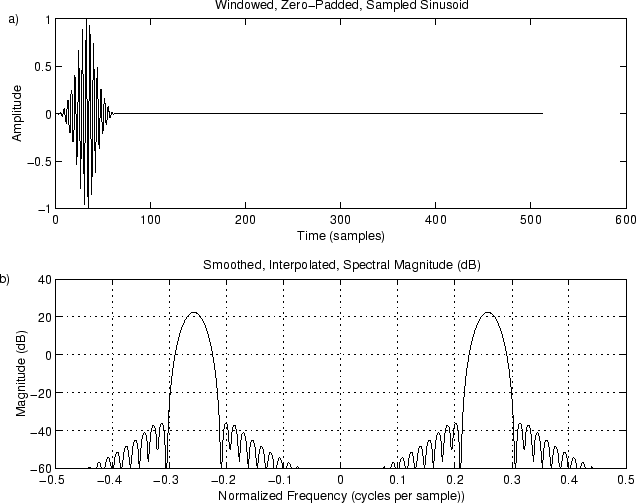
Example 5: Use of the Blackman Window

Now let's apply this window to the sinusoidal data:

% Use the Blackman window on the sinusoid data
xw = [w .* cos(2*pi*n*f*T),zeros(1,(zpf-1)*N)]; % windowed, zero-padded data
X = fft(xw);                                    % Smoothed, interpolated spectrum

% Plot time data
figure(6);
subplot(2,1,1);
plot(xw);     

title(‘Windowed, Zero-Padded, Sampled Sinusoid’);
xlabel(‘Time (samples)’); ylabel(’Amplitude’);
text(-50,1,‘a)’); hold off;

% Plot spectral magnitude in the best way
spec = 10*log10(conj(X).X);  % Spectral magnitude in dB
spec = max(spec,-60ones(1,nfft)); % clip to -60 dB
subplot(2,1,2);
plot(fninf,fftshift(spec),’-’); axis([-0.5,0.5,-60,40]); grid;
title(‘Smoothed, Interpolated, Spectral Magnitude (dB)’);
xlabel(‘Normalized Frequency (cycles per sample))’);
ylabel(‘Magnitude (dB)’);
text(-.6,40,‘b)’);
print -deps eps/xw.eps;

Figure 9.6:Effect of the Blackman window on the sinusoidal data segment.

<< Previous page  TOC  INDEX  Next page >>