Example 6: Hanning-Windowed Complex Sinusoid

NOTE: THIS DOCUMENT IS OBSOLETE, PLEASE CHECK THE NEW VERSION: "Mathematics of the Discrete Fourier Transform (DFT), with Audio Applications --- Second Edition", by Julius O. Smith III, W3K Publishing, 2007, ISBN 978-0-9745607-4-8. - Copyright © 2017-09-28 by Julius O. Smith III - Center for Computer Research in Music and Acoustics (CCRMA), Stanford University

<< Previous page  TOC  INDEX  Next page >>

Example 6: Hanning-Windowed Complex Sinusoid

In this example, we'll perform spectrum analysis on a complex sinusoidhaving only a single positive frequency. We'll use the Hanning window which does not have as much sidelobe suppression as the Blackman window, but its main lobe is narrower. Its sidelobes ''roll off'' very quickly versus frequency. Compare with the Blackman window results to see if you can see these differences.

% Example 5: Practical spectrum analysis of a sinusoidal signal

% Analysis parameters:
M = 31;         % Window length (we’ll use a “Hanning window”)
N = 64;         % FFT length (zero padding around a factor of 2)

% Signal parameters:
wxT = 2*pi/4;   % Sinusoid frequency in rad/sample (1/4 sampling rate)
A = 1;          % Sinusoid amplitude
phix = 0;       % Sinusoid phase

% Compute the signal x:
n = [0:N-1];    % time indices for sinusoid and FFT
x = A * exp(jwxTn+phix); % the complex sinusoid itself: [1,j,-1,-j,1,j,…]

% Compute Hanning window:
nm = [0:M-1];   % time indices for window computation
w = (1/M) * (cos((pi/M)*(nm-(M-1)/2))).^2;  % Hanning window = “raised cosine”

wzp = [w,zeros(1,N-M)]; % zero-pad out to the length of x
xw = x .* wzp;          % apply the window w to the signal x

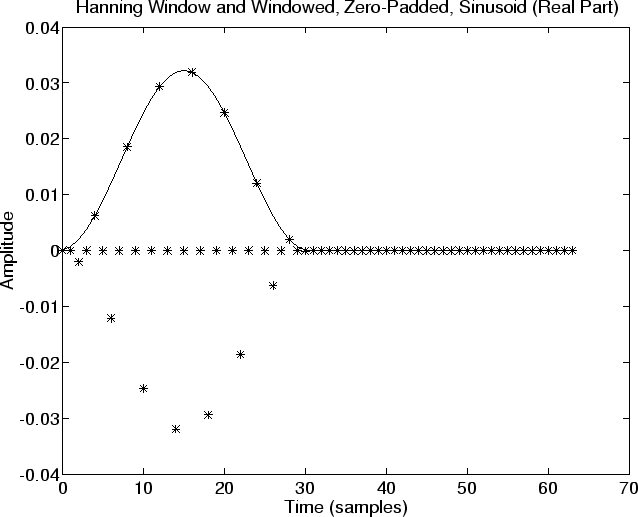
% Display real part of windowed signal and the Hanning window:
plot(n,wzp,’-’); hold on;
plot(n,real(xw),’’);
title(‘Hanning Window and Windowed, Zero-Padded, Sinusoid (Real Part)’);
xlabel(‘Time (samples)’); ylabel(‘Amplitude’); hold off;
disp ‘pausing for RETURN (check the plot). . .’; pause
print -deps eps/hanning.eps;

Figure 9.7:A length 31 Hanning Window (‘‘Raised Cosine’’) and the windowed sinusoid created using it. Zero-padding is also shown. The sampled sinusoid is plotted with `’ using no connecting lines. You must now imagine the continuous sinusoid threading through the asterisks.

% Compute the spectrum and its various alternative forms
%
Xw = fft(xw);              % FFT of windowed data
fn = [0:1.0/N:1-1.0/N];    % Normalized frequency axis
spec = 20log10(abs(Xw));  % Spectral magnitude in dB
% Since the zeros go to minus infinity, clip at -100 dB:
spec = max(spec,-100ones(1,length(spec)));
phs = angle(Xw);           % Spectral phase in radians
phsu = unwrap(phs);        % Unwrapped spectral phase (using matlab function)

To help see the full spectrum, we’ll also compute a heavily interpolated spectrum which we’ll draw using solid lines. (The previously computed spectrum will be plotted using ‘’.) Ideal spectral interpolation is done using zero-padding in the time domain:

Nzp = 16;                   % Zero-padding factor
Nfft = NNzp;               % Increased FFT size
xwi = [xw,zeros(1,Nfft-N)]; % New zero-padded FFT buffer
Xwi = fft(xwi);             % Take the FFT
fni = [0:1.0/Nfft:1.0-1.0/Nfft]; % Normalized frequency axis
speci = 20log10(abs(Xwi));      % Interpolated spectral magnitude in dB
speci = max(speci,-100ones(1,length(speci))); % clip at -100 dB
phsi = angle(Xwi);          % Phase
phsiu = unwrap(phsi);       % Unwrapped phase

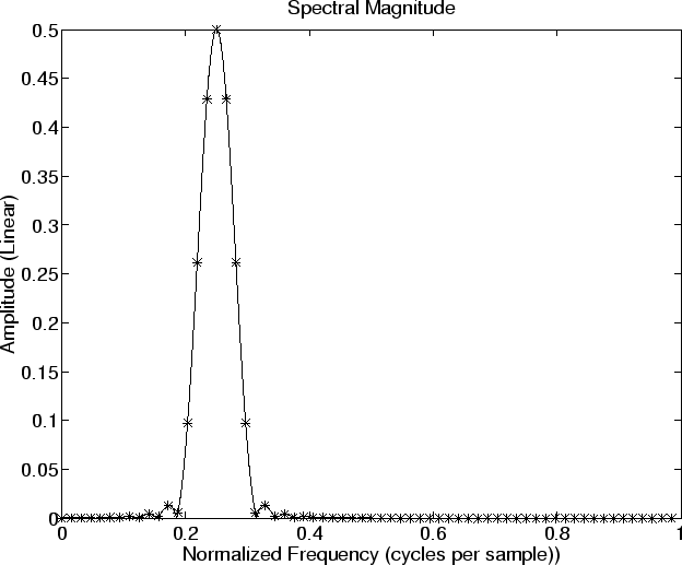
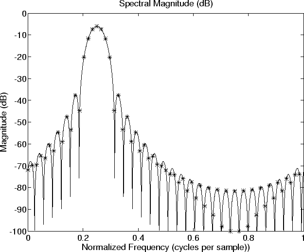
% Plot spectral magnitude
%
plot(fn,abs(Xw),’’); hold on; plot(fni,abs(Xwi));
title(‘Spectral Magnitude’);
xlabel(‘Normalized Frequency (cycles per sample))’);
ylabel(‘Amplitude (Linear)’);
disp ‘pausing for RETURN (check the plot). . .’; pause
print -deps eps/specmag.eps; hold off;

Figure 9.8:Spectral Magnitude, linear scale.

% Same thing on a dB scale
plot(fn,spec,’’); hold on; plot(fni,speci);
title(‘Spectral Magnitude (dB)’);
xlabel(‘Normalized Frequency (cycles per sample))’);
ylabel(‘Magnitude (dB)’);
disp ‘pausing for RETURN (check the plot). . .’; pause
print -deps eps/specmagdb.eps; hold off;

Figure 9.9:Spectral Magnitude, dB scale.

Note that there are no negative frequency components in Fig. 9.8because we are analyzing a complex sinusoid which is a sampled complex sinusoid frequency only.

Notice how difficult it would be to correctly interpret the shape of the ‘‘sidelobes’’ without zero padding. The asterisks correspond to a zero-padding factor of 2, already twice as much as needed to preserve all spectral information faithfully, but it is clearly not sufficient to make the sidelobes clear in a spectral magnitude plot.

---

Subsections

• Spectral Phase

<< Previous page  TOC  INDEX  Next page >>