Example 4: Blackman Window

NOTE: THIS DOCUMENT IS OBSOLETE, PLEASE CHECK THE NEW VERSION: "Mathematics of the Discrete Fourier Transform (DFT), with Audio Applications --- Second Edition", by Julius O. Smith III, W3K Publishing, 2007, ISBN 978-0-9745607-4-8. - Copyright © 2017-09-28 by Julius O. Smith III - Center for Computer Research in Music and Acoustics (CCRMA), Stanford University

<< Previous page  TOC  INDEX  Next page >>

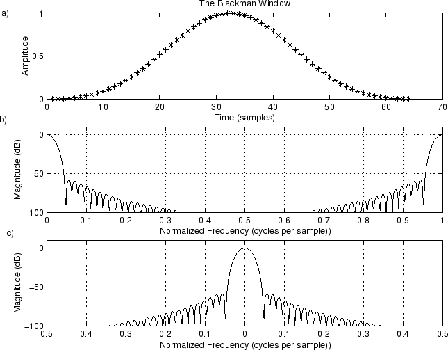
Example 4: Blackman Window

Finally, to finish off this sinusoid, let's look at the effect of using aBlackman window (which has nice but suboptimal parameters for audio work). Figure 9.5a shows the Blackman window, Fig. 9.5b shows its magnitude spectrum on a dB scale, and Fig. 9.5c introduces the use of a more natural frequency axis which interprets the upper half of the bin numbers as negative frequencies. Here is the Matlab for it:

% Add a "Blackman window"
% w = blackman(N); % if you have the signal processing toolbox
w = .42-.5*cos(2*pi*(0:N-1)/(N-1))+.08*cos(4*pi*(0:N-1)/(N-1));
figure(5);
subplot(3,1,1); plot(w,'*'); title('The Blackman Window');
xlabel('Time (samples)'); ylabel('Amplitude');
text(-8,1,'a)'); 

% Also show the window transform:
xw = [w,zeros(1,(zpf-1)N)]; % zero-padded window (col vector)
Xw = fft(xw);                 % Blackman window transform
spec = 20log10(abs(Xw));     % Spectral magnitude in dB
spec = spec - max(spec);      % Usually we normalize to 0 db max
spec = max(spec,-100*ones(1,nfft)); % clip to -100 dB
subplot(3,1,2); plot(fni,spec,’-’); axis([0,1,-100,10]); grid;
xlabel(‘Normalized Frequency (cycles per sample))’);
ylabel(‘Magnitude (dB)’);
text(-.12,20,‘b)’);

% Replot interpreting upper bin numbers as negative frequencies:
nh = nfft/2;
specnf = [spec(nh+1:nfft),spec(1:nh)];  % see also Matlab’s fftshift()
fninf = fni - 0.5;
subplot(3,1,3);
plot(fninf,specnf,’-’); axis([-0.5,0.5,-100,10]); grid;
xlabel(‘Normalized Frequency (cycles per sample))’);
ylabel(‘Magnitude (dB)’);
text(-.6,20,‘c)’);
print -deps eps/blackman.eps;

Figure 9.5:The Blackman Window. a) The window itself in the time domain. b) DB Magnitude spectrum. c) DB magnitude spectrum plotted over frequencies .

<< Previous page  TOC  INDEX  Next page >>