NOTE: THIS DOCUMENT IS OBSOLETE, PLEASE CHECK THE NEW VERSION: "Mathematics of the Discrete Fourier Transform (DFT), with Audio Applications --- Second Edition", by Julius O. Smith III, W3K Publishing, 2007, ISBN 978-0-9745607-4-8. - Copyright © 2017-09-28 by Julius O. Smith III - Center for Computer Research in Music and Acoustics (CCRMA), Stanford University
<< Previous page TOC INDEX Next page >>
The Analytic Signal and Hilbert Transform Filters
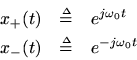
A signal which has no negative-frequency components is called ananalytic signal.5.6 Therefore, in continuous time, every analytic signal
can be represented as
whereis the complex coefficient (setting the amplitude and phase) of the positive-freqency complex sinusoid
atfrequency
.
Any sinusoid
in real life may be converted to a positive-frequency complex sinusoid
by simply generating a phase-quadrature component
to serve as the ''imaginary part'':
The phase-quadrature component can be generated from the in-phase componentby a simple quarter-cycle time shift.5.7For more complicated signals which are expressible as a sum of many sinusoids, a filter can be constructed which shifts each sinusoidal component by a quarter cycle. This is called a Hilbert transform filter. Let
denote the output at time
of theHilbert-transform filter applied to the signal
. Ideally, this filter has magnitude
at all frequencies and introduces a phase shift of
at each positive frequency and
at each negative frequency. When a real signal
and its Hilbert transform
are used to form a new complex signal
, the signal
has the property that all ''negative frequencies'' of
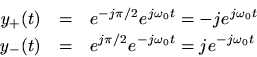
To see how this works, recall that these phase shifts can be impressed on a complex sinusoid by multiplying it by
. Consider the positive and negative frequency components at the particular frequency
:
Now let's apply adegrees phase shift to the positive-frequency component, and a
degrees phase shift to the negative-frequency component:
Adding them together gives
and sure enough, the negative frequency component is filtered out. (There is also a gain of 2 at positive frequencies which we can remove by defining the Hilbert transform filter to have magnitude 1/2 at all frequencies.)For a concrete example, let's start with the real sinusoid
Applying the ideal phase shifts, the Hilbert transform is
The analytic signal is then
by Euler's identity. Thus, in the sum, the negative-frequency components of
cancel out in the sum, leaving only the positive-frequency component. This happens for any real signal
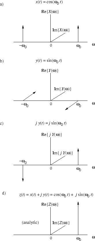
Figure 5.8:Creation of the analytic signal from the real sinusoid
and the derived phase-quadrature sinusoid
, viewed in the frequency domain. a) Spectrum of
. b) Spectrum of
. c) Spectrum of
. d) Spectrum of
.
Figure 5.8 illustrates what is going on in the frequency domain. While we haven't ''had'' Fourier analysis yet, it should come as no surprise that the spectrum of a complex sinusoid
will consist of a single ''spike'' at the frequency
and zero at all other frequencies. (Just follow things intuitively for now, and revisit Fig. 5.8 after we've developed the Fourier theorems.) From the identity
, we see that the spectrum contains unit-amplitude ''spikes'' at
. Similarly, the identity
says that we have an amplitude
spike at
spike at
by
results in
which is a unit-amplitude ''up spike'' at
), and the negative-frequency up-spike in the cosine iscanceled by the down-spike in
. This sequence of operations illustrates how the negative-frequency component
gets filtered outby the addition of
and
.
As a final example (and application), let
, where
is a slowly varying amplitude envelope (slow compared with
5.8, and the analytic signal is
. Note that AM demodulation5.9 is now nothing more than the absolute value. I.e.,
. Due to this simplicity, Hilbert transforms are sometimes used in makingamplitude envelope followers for narrowband signals (i.e., signals with all energy centered about a single ''carrier'' frequency). AM demodulation is one application of a narrowband envelope follower.