NOTE: THIS DOCUMENT IS OBSOLETE, PLEASE CHECK THE NEW VERSION: "Mathematics of the Discrete Fourier Transform (DFT), with Audio Applications --- Second Edition", by Julius O. Smith III, W3K Publishing, 2007, ISBN 978-0-9745607-4-8. - Copyright © 2017-09-28 by Julius O. Smith III - Center for Computer Research in Music and Acoustics (CCRMA), Stanford University

<< Previous page  TOC  INDEX  Next page >>

Signal Metrics

This section defines some useful functions of signals.

The mean of a signal (more precisely the ''sample mean'') is defined as its average value:

The total energy of a signal is defined the sum of squaredmoduli:

Energy is the ''ability to do work.'' In physics, energy and work are in units of ''force times distance,'' ''mass times velocity squared,'' or other equivalent combinations of units. The energy of a pressure wave is the integral over time of the squared pressure divided by the wave impedance the wave is traveling in. The energy of a velocity wave is the integral over time of the squared velocity times the wave impedance. In audio work, a signal is typically a list of pressure samplesderived from a microphone signal, or it might be samples of forcefrom a piezoelectric transducer, velocity from a magnetic guitarpickup, and so on. In all of these cases, the total physical energy associated with the signal is proportional to the sum of squared signal samples. (Physical connections in signal processing are explored more deeply in Music 421.)

The average power of a signal is defined the energy per sample:

Another common description when is real is the ''mean square.'' When is a complex sinusoid, i.e., , then ; in other words, for complex sinusoids, the average power equals the instantaneous power which is the amplitude squared.

Power is always in physical units of energy per unit time. It therefore makes sense to define the average signal power as the total signal energydivided by its length. We normally work with signals which are functions of time. However, if the signal happens instead to be a function of distance (e.g., samples of displacement along a vibrating string), then the ''power'' as defined here still has the interpretation of a spatial energy density. Power, in contrast, is a temporal energy density.

The root mean square (RMS) level of a signal is simply . However, note that in practice (especially in audio work) an RMS level may be computed after subtracting out the mean value. Here, we call that the variance.

The variance (more precisely the sample variance) of the signal is defined as the power of the signal with its sample mean removed:

It is quick to show that, for real signals, we have

which is the ''mean square minus the mean squared.'' We think of the variance as the power of the non-constant signal components (i.e., everything but dc). The terms ''sample mean'' and ''sample variance'' come from the field of statistics, particularly the theory of stochastic processes. The field of statistical signal processing[16] is firmly rooted in statistical topics such as ''probability,'' ''random variables,'' ''stochastic processes,'' and ''time series analysis.'' In this course, we will only touch lightly on a few elements of statistical signal processing in a self-contained way.

The norm of a signal is defined as the square root of its total energy:

We think of as the length of in -space. Furthermore, is regarded as the distance between and . The norm can also be thought of as the ''absolute value'' or ''radius'' of a vector.^6.2

Example: Going back to our simple 2D example , we can compute its norm as . The physical interpretation of the norm as a distance measure is shown in Fig. 6.5.

Figure 6.5:Geometric interpretation of a signal norm in 2D.

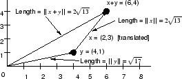
Example: Let's also look again at the vector-sum example, redrawn in Fig. 6.6.

Figure 6.6:Length of vectors in sum.

The norm of the vector sum is

while the norms of and are and , respectively. We find that which is an example of the triangle inequality. (Equality occurs only when and are colinear, as can be seen geometrically from studying Fig. 6.6.)

Example: Consider the vector-difference example diagrammed in Fig. 6.7.

Figure 6.7:Length of a difference vector.

The norm of the difference vector is

---

Subsections

• Other Norms

<< Previous page  TOC  INDEX  Next page >>