NOTE: THIS DOCUMENT IS OBSOLETE, PLEASE CHECK THE NEW VERSION: "Mathematics of the Discrete Fourier Transform (DFT), with Audio Applications --- Second Edition", by Julius O. Smith III, W3K Publishing, 2007, ISBN 978-0-9745607-4-8. - Copyright © 2017-09-28 by Julius O. Smith III - Center for Computer Research in Music and Acoustics (CCRMA), Stanford University
<< Previous page TOC INDEX Next page >>
The Complex Plane
We can plot complex numbers
in a plane as ordered pairs
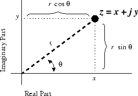
, as shown in Fig. 2.2. The complex plane is any 2D graph in which the horizontal axis is the real part and the vertical axis is the imaginary part of a complex number or function. As an example, the number
has coordinates
in the complex plane while the number
has coordinates
.
Plotting
, where
is the distance from the origin
to the number being plotted, and
is the angle of the number relative to the positive real coordinate axis (the line defined by
and
). (See Fig. 2.2.)
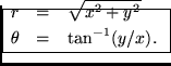
Using elementary geometry, it is quick to show that conversion from rectangular to polar coordinates is accomplished by the formulas
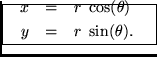
The first equation follows immediately from the Pythagorean theorem, while the second follows immediately from the definition of the tangent function. Similarly, conversion from polar to rectangular coordinates is simplyThese follow immediately from the definitions of cosine and sine, respectively,